LFExplained

The first time I learned about the inner workings of the lfe package in R, I was told to read a paper by mathematician Israel Halperin called “The product of projection operators” (good luck finding it though. The only reason why I was able to access it is because I was sent a pdf at one point). This paper is concerned with generalizing a technique known as the method of alternating projections. Von Neumann first proved that by successively projecting a vector into two affine spaces, you converge on the projection into their intersection. Halperin managed to extend this result to remarkable generality, only requiring some minimal Banach space structure. I dutifully read this paper, but remember very little about the details. The level of generality was simply more than I really cared to take the time to understand, especially since my interest in it only went as far as understanding how an R package works.

It occurred to me recently that while the Halperin paper is difficult to grasp even at a conceptual level, the original von Neumann approach is so simple that extending it to an arbitrary number of projections in Euclidean space should be doable by fairly elementary means. Like most things I write, this probably won’t be of any use for the practitioner, except maybe to impart a sense of awe the next time a 20-way felm runs in mere minutes.

First some background. When I was first taught about the Frisch-Waugh-Lovell theorem, it was mostly framed as a formal justification for “adding controls” to linear regression models as a way to remove the confounding effects of other covariates. LFE uses the theorem in a completely different way: as a computational tool to speed up regressions. As a review, suppose we have a regression model:

$Y = X_1'\beta_1 + X_2'\beta_2 + \varepsilon$

Let $\mathbb X = [\mathbb X_1\ \mathbb X_2]$ be the partitioned design matrix. Then by the usual OLS, we have:

$\begin{bmatrix}\hat\beta_1 \\ \hat\beta_2\end{bmatrix} = (\mathbb X'\mathbb X)^{-1} \mathbb X'\mathbb Y$

One version of Frisch-Waugh-Lovell tells us that an alternative expression for $\hat\beta_1$ is given by:

$\hat\beta_1 = \left(\widehat{\mathbb X}_1' \widehat{\mathbb X}_1\right) \widehat{\mathbb X}_1\mathbb Y$

where

$\widehat{\mathbb X}_1 = \mathbb M_2 \mathbb X_1 = \left(\mathbb I - \mathbb X_2(\mathbb X_2'\mathbb X_2)^{-1}\mathbb X_2'\right) \mathbb X_1$

$\mathbb M_2$ is often known as the “residual maker” matrix because when applied to a vector $\mathbb A = [A_1,A_2,\ldots,A_n]'$ , it returns the residuals from an OLS regression of $X_2$ on $A$ . I leave a few elementary properties as an exercise:

Exercise 1:

$\mathbb M_2$ is idempotent, i.e. $\mathbb M_2 \mathbb M_2 = \mathbb M_2$
$\mathbb M_2$ is symmetric, i.e. $\mathbb M_2' = \mathbb M_2$
Conclude from above that $\mathbb M_2 = QDQ'$ where $Q$ is an orthonormal matrix and $D = \begin{bmatrix} 1 & \cdots & \cdots & \cdots & \cdots & 0\\ \vdots & \ddots & \ddots & \ddots & \ddots & \vdots\\ \vdots & \ddots & 1 & \ddots & \ddots & \vdots\\ \vdots & \ddots & \ddots & 0 & \ddots & \vdots\\ \vdots & \ddots & \ddots & \ddots & \ddots & \vdots\\ 0& \cdots & \cdots & \cdots & \cdots & 0\end{bmatrix}$
Additionally, if $X_2 \in \mathbb R^p$ is not collinear, then there are exactly $n - p$ 1’s in the above.

(Side note: typing that matrix was not fun).

screen shot 2019-01-16 at 7.35.40 pm — Keeping with the theme of only using ridiculous pictures

In particular, because of the above properties, $\mathbb M_2$ is a projection matrix and therefore has the special property there is some $n-p$ dimensional subspace of $\mathbb R^n$ , $S$ such that $\mathbb M_2 s = s\,\forall s\in S$ and $\mathbb M_2 t = s^* = \mathrm{argmin}_{s\in S} |t - s|$ . In fact, the subspace is exactly the span of the first $n-p$ columns of $Q$ (uh, it might be the first rows, I can never remember this).

The sorts of models lfe excels at are ones of the form

$Y = X_1'\beta + F_1'\delta_1 + \cdots + F_k'\delta_k + \varepsilon$

where each $F_j$ has the special property that it is a $q_j \times 1$ dimensional vector such that exactly one entry is 1 and the rest are 0. Intuitively, we can think of the $F_j$ as categories such that belonging in a given category has the effect of shifting the regression function up or down by some amount $\delta_{mj}$ . The shifts associated with the $F$ ‘s are known as fixed effects, and econometricians often just write as shorthand:

$Y = X_1'\beta + \delta_{j_1} + \cdots + \delta_{j_k} + \varepsilon$

Exercise 2: Show that $\left(\mathbb M_{F_j} \mathbb X\right)_i = X_i - \bar X_{j,m}$ where $\bar X_{j,m}$ is the average value of $X$ among those observations where $F_j$ has a 1 in its $m^{th}$ component. This is known as de-meaning

The fixed effects are usually not the parameters of interest, so we would like to estimate $\hat\beta_1$ without estimating all of the fixed effects if possible. The power of lfe comes from its ability to abuse this fact. Demeaning in this manner is considerably more efficient than building out the entire design matrix and inverting its covariance matrix (or more realistically, doing QR decomposition with something like a Householder transformation or a Given’s rotation for numerical stability). In the case where $k = 1$ , we now have a complete description of what lfe does. It simply demeans and then regresses using the de-meaned variables. What happens when $k > 1$ ? In this case, we need to project into the space associated with $F = [F_1,F_2,\ldots,F_k]$ . Unfortunately, it is not obvious how to project into this space. The demeaning formula no longer works and it is once again unclear how to do the projection without building up a huge design matrix. We will now need one more fact to finally motivate the use of the method of alternating projections.

Exercise 3: Show that if $\mathbb M_{F_j}$ projects into $S_j$ , then $\mathbb M_F$ is the orthogonal projection into $S_1 \cap S_2 \cap \cdots \cap S_k$ .

So at this point we know how to project into each individual $S_j$ easily, but we want to efficiently project into the intersection. In fact, the von Neumann result already shows us that if $k = 2$ , then $\lim_{n\to\infty} (\mathbb M_{F_1} \mathbb M_{F_2})^n = \mathbb M_F$ .

fig2caption — Visual intuition for the von Neumann result. Photo from here

The natural next question then is: does $\lim_{n\to\infty} \left(\mathbb M_{F_1} \cdots M_{F_k}\right)^n \to \mathbb M_F$ ? The answer will turn out to be yes. Let us first express this in slightly more abstract terms. Essentially, we want to prove the following:

Theorem 4: Suppose $A_1,\ldots,A_k \in \mathbb R^{d\times d}$ are orthogonal projection matrices into spaces $S_1,\ldots,S_k$ . Then $\lim_{n\to\infty} (A_1\cdots A_k)^n = A$ where $A$ is the orthogonal projection into the space $S_1\cap\cdots\cap S_k$ .

Orthogonality is a bit annoying to deal with, so let’s begin by proving something slightly easier.

Theorem 5: Suppose $A_1,\ldots,A_k \in \mathbb R^{d\times d}$ are projection matrices into spaces $S_1,\ldots,S_k$ . Then $\lim_{n\to\infty} (A_1\cdots A_k)^n = A$ where $A$ is a projection into the space $S_1\cap\cdots\cap S_k$ .

For notational convenience, call $A_1 \cdots A_k = A^*$ and $S_1\cap\cdots\cap S_k = S$ . First, note that $A^* s = s$ for all $s\in S$ , so $\lim_{n\to\infty} (A^*)s = s$ . We next show that $A$ is well defined for vectors not in $S$ and has image $S$ . This will show that $A$ is a projection. Let $S$ be $m$ dimensional and extend an orthonormal basis on $S$ , $s_1,\ldots,s_m$ to an orthonormal basis on $\mathbb R^n$ given by $s_1,\ldots,s_m,t_{m+1},\ldots,t_d$ . It will suffice to show that any $t = \sum_{i=m+1}^d \lambda_i t_i$ has $||(A^*)^n t - s|| \to 0$ for some $s \in S$ (this will simultaneously show the existence of $A$ and that its range is $S$ . Recall that the operator norm for a matrix is given by $||M|| = \sup_{||x||\leq 1} ||Mx||$ . The idea for the rest of the proof is now fairly straightforward. Because $A_j$ are all projections, the size of $\sum_{i=m+1}^d \lambda_i t_i$ can never go up. Furthermore, because we are in a finite dimensional space (the lack of finite dimensions is why the Halperin paper has to use much less elementary techniques), we can bound this shrinkage factor away from 1. But in doing so, we immediately get an exponential estimate on the rate of convergence.

Exercise 6: For a nontrivial projection matrix $M (\neq 0)$ , show that $||M|| = 1$ and the supremum is attained if and only if $x = Mx$ .

Since each $t_i$ is not in $S_j$ for some $j$ , then there is some first index such that $A_j t_j \neq t_j$ . Let $\mu_i = ||A_j t_i|| < 1$ . Then $A^* t_i < \mu_i$ . Let $\mu = \max_i \mu_i < 1$ . It is then clear that for any vector $t = \sum_{i=m+1}^d \lambda_i t_i$ , we have $\frac{||A^* t||}{||t||} \leq \mu$ . Now fix some such $t$ and consider the sequence $(A^*)^n t$ . If $(A^*)^p t \in S$ for some $p$ , then we must have $(A^*)^q t = (A^*)^p t$ for all $p \geq q$ by the above discussion. But then we are immediately done since then $(A^*)^n t \to (A^*)^q t \in S$ . With the orthonormal basis we constructed before, we must have $(A^*)^n t = \sum_{i=1}^m \lambda_i^n s_i^n + \sum_{i=m+1}^d \lambda_i^n t_i^n$ (the $n$ ‘s on the RHS are superscripts, not exponents). Define $\tau_n = \sum_{i=m+1}^d \lambda_i^n t_i^n$ and $\sigma_n = \sum_{i=1}^m \lambda_i^n s_i^n$ .

Exercise 7: Show that $||\tau_n|| \leq \mu||\tau_{n-1}||$ and $||\sigma_n - \sigma_{n-1}|| \leq ||\tau_n||$ . Use this to conclude that $(A^*)^n t \to s$ for some $s\in S$ as desired, completing the proof of theorem 5.

We now add the orthogonality back in. All we need to do is show that if each $A_j$ is orthogonal, then $A t_i = 0$ . It will suffice to show that $A_j t_i \notin S$ for each $j$ (since in this case, $\sigma_n = 0$ using the notation of exercise 7). But another change of basis makes this easy. Extend $s_1,\ldots,s_m$ to an orthonormal basis $u_{m+1}\ldots u_{r_j},v_{r_j+1},\ldots,v_d$ where $r_j$ is the rank of $A_j$ , and $\mathrm{span}(s_1,\ldots,u_{r_j}) = \mathrm{Range}(A_j)$ . Then $A_j \left(\sum \nu_k s_k + \sum \nu_k u_k + \sum \nu_i v_i\right) = \sum \nu_i s_i + \sum \nu_i u_i$ by orthogonality of $A_j$ . Additionally, $t_i = \sum \nu_k u_k + \sum \nu_k v_k$ (since it is orthogonal to $S$ ). Then $A_j \sum t_i = \sum \nu_k u_k \notin S$ .

In fact, as mentioned earlier, we have shown something even more remarkable.

Corollary 8: $d((A^*)^n,S) = O\left(e^{-n}\right)$ .

The rate of convergence of the alternating projections is at least linear. Roughly speaking, linear convergence means that there are some $c,C$ such that if we want $k$ digits of precision, then we need to iterate at most $C k$ times and at least $ck$ times. Assuming the $\mu$ from the above proof stays constant, we can now analyze the time complexity of felm fairly closely. Let $n_f$ be the number of fixed effects, $tol$ be the desired number of digits of precision, $n_p$ be the number of parameters of interest, and $N$ be the size of the data. Demeaning is an $O(N)$ operation and we have to do it $n_f$ times per iteration. By the linearity of convergence, we have that we need to project $O(tol)$ times. At the end, we have to do normal OLS on the demeaned data, which is $O(N n_p^2)$ Thus, we have that the time complexity of felm is $O(N(n_ftol + n_p^2))$ , so adding fixed effects incurs only a linear cost. By contrast, naive OLS on the entire system of fixed effects directly is $O(N(p_n + p_f)^2)$ , so it will grow quadratically in the number of “ways” of our fixed effects.

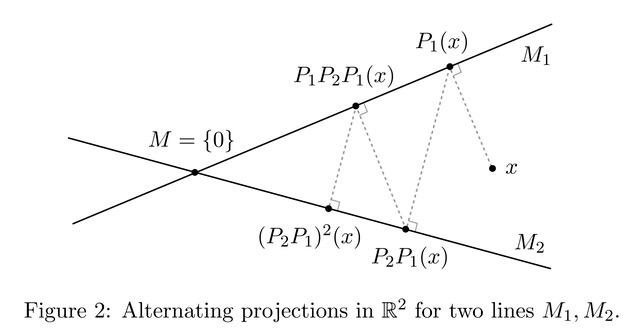
In hindsight, none of these facts should be particularly surprising. The visual intuition from figure 2 is the main insight, and we’ve just been playing around the symbols to fill in the technical details. Even the rate of convergence should not be terribly surprising. Alternating projections just repeatedly multiplying a matrix that is “<1” in some sense by itself repeatedly. Doing this with a real number <1 gives exactly linear convergence, so it is unsurprising that this extends to matrices with the proper construction.

I conclude by musing that this sort of proof is really only something that makes sense to publish in some sort of informal setting such as a blog. For those more interested in the theoretical aspects of the projections, there is little reason to not just read the Halperin paper. It doesn’t draw on any particularly deep math, is considerably more general, and is much more representative of the functional analytic tools of the trade necessary for further exploration. On the other hand, for the practitioner, there is little value added in knowing the gory details of the proof. In this case, I doubt knowledge about why alternating projections works would even be useful for debugging unexpected lfe behavior. Nonetheless, I hope I have impressed upon you some of the beauty and elegance of the inner workings of my most used R package.

Bonus Exercise: The derivation of FWL purely from matrix algebra is tedious/intimidating, but straightforward. This is not my favorite proof of FWL (my favorite can be found in Theorem 2.1 here), but I think it is still informative in its own right and worth doing exactly one time in your life. I will outline it here. Using the notations from earlier, we have:

$(\mathbb X'\mathbb X)^{-1}\mathbb X' \mathbb Y = \begin{bmatrix}\mathbb X_1'\mathbb X_1 & \mathbb X_1' \mathbb X_2 \\ \mathbb X_2'\mathbb X_1 & \mathbb X_2'\mathbb X_2\end{bmatrix}^{-1}\begin{bmatrix}\mathbb X_1'\mathbb Y \\ \mathbb X_2'\mathbb Y\end{bmatrix}$

The main difficulty in getting something more tractable is inverting the partitioned matrix. Fortunately, manipulating partitioned matrices is an extremely well studied problem. Let

$M = \begin{bmatrix}A & B \\ C & D\end{bmatrix}$

and define $M/D = A-BD^{-1}C$ and $M/A = D - CA^{-1} B$ . Show the Shur complement formula:

$\begin{bmatrix}(M/D)^{-1} & -(M/D)^{-1}BD^{-1} \\ -D^{-1}C(M/D)^{-1} & (M/A)^{-1}\end{bmatrix}$

(Hint: the proof is not hard, only tedious. The only trick is to write

$\begin{bmatrix}A & B \\ C & D\end{bmatrix} \begin{bmatrix}E & F \\ G & K\end{bmatrix} = \begin{bmatrix}\mathbb I & 0 \\ 0 & \mathbb I\end{bmatrix}$

and then solve/simplify). Now, use the Shur complement formula to show

$\hat\beta_1 = \left(\mathbb X_1' \mathbb M_2 \mathbb X_1\right)^{-1}\mathbb X_1' \mathbb M_2 \mathbb Y$

(Hint: the idempotency of $\mathbb M_2$ is your friend). Finally, use idempotency once more to get the form of the FWL theorem I stated in the post:

$\hat\beta_1 = \left(\widehat{\mathbb X}_1' \widehat{\mathbb X}_1\right) \widehat{\mathbb X}_1\mathbb Y$

LFExplained

Published by statsmodel

Leave a comment Cancel reply

Share this:

Related

Published by statsmodel

Leave a comment Cancel reply